Spherical Harmonics

Marc R. Roussel

Department of Chemistry and Biochemistry

University of Lethbridge

Definition and normalization

The purpose of this document is to investigate the spherical harmonics and to learn how to use them in quantum mechanical problems. The following commands define the spherical harmonics. There's some slightly mysterious stuff in there that you shouldn't worry about.

>	_EnvLegendreCut := 1..infinity:

>	LPct := (l,m,theta) -> LegendreP(l,abs(m),cos(theta));

>	NF := proc(l,m) local theta; 1/sqrt(int(LPct(l,m,theta)^2*sin(theta),theta=0..Pi)); end proc;

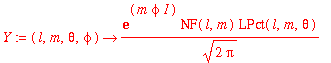
>	Y := (l,m,theta,phi) -> exp(I*m*phi)/sqrt(2*Pi)*NF(l,m)*LPct(l,m,theta);

Let's start by verifying that these are normalized by doing a few examples:

>	int(int(conjugate(Y(0,0,theta,phi))*Y(0,0,theta,phi)*sin(theta),theta=0..Pi),phi=0..2*Pi);

Note the explicit complex-conjugate operation and the factor of sin( theta) in the integral which comes from the volume element.

>	int(int(conjugate(Y(1,0,theta,phi))*Y(1,0,theta,phi)*sin(theta),theta=0..Pi),phi=0..2*Pi);

>	int(int(conjugate(Y(1,1,theta,phi))*Y(1,1,theta,phi)*sin(theta),theta=0..Pi),phi=0..2*Pi);

Visualization

Let's see what these things look like. We have a small problem to overcome: These functions are complex-valued. You can't easily plot complex numbers. We have a number of options, but perhaps the simplest is to plot Y^*Y (i.e. |Y|^2). The probability density is what we're interested in most of the time anyway. Let's start by defining the probability density. This is most easily done by hand.

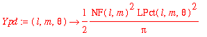
>	Ypd := (l,m,theta) -> 1/(2*Pi)*NF(l,m)^2*LPct(l,m,theta)^2;

Note that it only depends on theta. In other words, the probability density is symmetric with respect to rotations around the z  axis. To get an idea of what the probability density looks like as a function of theta, we use a polar plot. In this type of plot, the distance from the origin indicates the value of the function. Here first is the l =0, m =0 harmonic:

>	plot([Ypd(0,0,theta),theta,theta=0..2*Pi],-0.1..0.1,-0.1..0.1,coords=polar);

l =1, m =0:

>	plot([Ypd(1,0,theta),theta,theta=0..2*Pi],-0.3..0.3,-0.1..0.1,coords=polar,scaling=CONSTRAINED);

l =1, m =1:

>	plot([Ypd(1,1,theta),theta,theta=0..2*Pi],-0.1..0.1,-0.15..0.15,coords=polar,scaling=CONSTRAINED);

l =2, m =0:

>	plot([Ypd(2,0,theta),theta,theta=0..2*Pi],-0.45..0.45,-0.12..0.12,coords=polar,scaling=CONSTRAINED);

l =2, m =1:

>	plot([Ypd(2,1,theta),theta,theta=0..2*Pi],-0.15..0.15,-0.15..0.15,coords=polar,scaling=CONSTRAINED);

l =2, m =2:

>	plot([Ypd(2,2,theta),theta,theta=0..2*Pi],-0.1..0.1,-0.2..0.2,coords=polar,scaling=CONSTRAINED);

To see what these shapes look like in 3-d, you have to imagine rotating them around the z  axis which corresponds to the horizontal axis in these pictures. We can actually do this with Maple:

>	with(plots):

Warning, the name changecoords has been redefined

Let's look at the 2,0 spherical harmonic. The z  axis is pointing toward the top of the page.

>	sphereplot(Ypd(2,0,theta),phi=0..2*Pi,theta=0..Pi,orientation=[150,90]);

Here's the 2,1 harmonic, in a projection in which the z  axis is tilted slightly towards us:

>	sphereplot(Ypd(2,1,theta),phi=0..2*Pi,theta=0..Pi,orientation=[0,65]);

Finally, here's the 2,2, in the same orientation as the previous harmonic:

>	sphereplot(Ypd(2,2,theta),phi=0..2*Pi,theta=0..Pi,orientation=[0,65]);

Expectation values

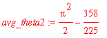
We can work out expectation values more or less as we have done before, except that we need to be careful about the volume element and complex-conjugate operation. Suppose for example that we want to calculate the standard deviation of theta for l =2, m =0. To do that, we need < theta> and < theta^2>.

>	avg_theta := int(int(conjugate(Y(2,0,theta,phi))*theta*Y(2,0,theta,phi)*sin(theta),theta=0..Pi),phi=0..2*Pi);

>	avg_theta2 := int(int(conjugate(Y(2,0,theta,phi))*theta^2*Y(2,0,theta,phi)*sin(theta),theta=0..Pi),phi=0..2*Pi);

>	Delta_theta := sqrt(avg_theta2-avg_theta^2);