Chemistry 2720 Fall 2000 Assignment 6 Solutions

1.

We must first convert kJ/mol to J (per photon):

$$E = \frac{239.2\times 10^3\,\mathrm{J/mol}}{6.022\,142\times 10^{23}\,\mathrm{mol}^{-1}} = 3.972\times 10^{-19}\,\mathrm{J}.$$

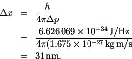
Since $E = h\nu$, we have

$$\nu = \frac{E}{h} = \frac{3.972\times 10^{-19}\,\mathrm{J}}{6... ...s 10^{-34}\,\mathrm{J/Hz}} = 5.995\times 10^{14}\,\mathrm{Hz}.$$

This is in the yellow-green region of the visible spectrum.

2.

The uncertainty in the momentum is

$$\Delta p = m\Delta v = (1.674\,927\times 10^{-27}\,\mathrm{kg})(1\,\mathrm{m/s}) = 1.675\times 10^{-27}\,\mathrm{kg\,m/s}.$$

The minimum uncertainty in the position is therefore

$$\begin{eqnarray*}\Delta x & = & \frac{h}{4\pi\Delta p}\\ & = & \frac{6.626\,06... ...75\times 10^{-27}\,\mathrm{kg\,m/s}}\\ & = & 31\,\mathrm{nm}. \end{eqnarray*}$$

3.

(a)

The wavelength is

$$\lambda = \left(\frac{\Delta r}{0.7C_s^{1/4}}\right)^{4/3} =... ...hrm{m})^{1/4}}\right)^{4/3} = 2.56\times 10^{-12}\,\mathrm{m}.$$

Given the wavelength, we can calculate the momentum:

$$p = \frac{h}{\lambda} = 2.59\times 10^{-22}\,\mathrm{kg\,m/s}.$$

(b)

$$\begin{eqnarray*}% latex2html id marker 52 E^2 & = & c^2p^2 + m_0^2c^4\\ & = &... ...hrm{J}^2\\ \therefore E & = & 1.13\times 10^{-13}\,\mathrm{J} \end{eqnarray*}$$

(c)

The kinetic energy (K) is

$$\begin{eqnarray*}K & = & E - m_0c^2\\ & = & 1.13\times 10^{-13}\,\mathrm{J} - ... ...10^8\,\mathrm{m/s})^2\\ & = & 3.11\times 10^{-14}\,\mathrm{J} \end{eqnarray*}$$

But K = eV so that

$$V = \frac{K}{e} = \frac{3.11\times 10^{-14}\,\mathrm{J}}{1.602\,176\times 10^{-19}\,\mathrm{C}} = 194\,\mathrm{kV}.$$

4.

(a)

This is a straightforward application of the Bragg equation $n\lambda = 2d\sin\theta$ with n=1:

$$d = \frac{\lambda}{2\sin\theta}$$

For example, the first line gives us

$$d = \frac{70.8\,\mathrm{pm}}{2\sin(6.6^\circ)} = 308\,\mathrm{pm}.$$

Here is a complete table of results:

$\theta$ (degrees)	6.6	9.2	11.4	13.1	14.7
d (pm)	308	221	179	156	140

(b)

The first reflection is probably the (100), so $a = d_{100} \approx 308\,\mathrm{pm}$. We then manipulate the equation for the interplane distances:

h² + k² + l² = (a/d_hkl)².

If we were right about the first reflection being the (100) interplane distance, we should be able to determine the Miller indices corresponding to each of the other reflections by computing the approximate sum of their squares by the above formula and then finding a consistent set of indices by trial-and-error:

dhkl (pm)	221	179	156	140
h2+k2+l2	2	3	4	5
(hkl)	(110)	(111)	(200)	(210)

Now that we know the Miller indices, we can calculate a = d_hkl(h²+k²+l²)^1/2 from each reflection and average the results.

(hkl)	(100)	(110)	(111)	(200)	(210)
dhkl (pm)	308	221	179	156	140
a (pm)	308	313	310	312	313

The average is therefore $311\,\mathrm{pm}$.

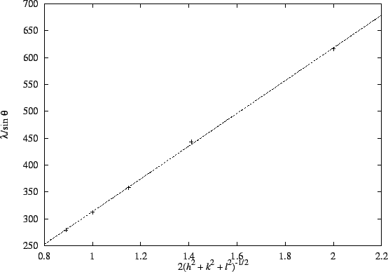
The better method is to combine the equation for the interplane distances with the Bragg condition. We get

$$\frac{\lambda}{\sin\theta} = a\frac{2}{(h^2+k^2+l^2)^{1/2}}.$$

Thus, a plot of $\lambda/\sin\theta$ vs 2(h²+k²+l²)^-1/2 should have a slope of a and an intercept near zero. Note that the standard linear regression method implemented in (e.g.) calculators assumes that the abscissas are error-free while the ordinates contain random errors so that the above-described plot is, of all the possible ways of plotting the data, a statistically correct choice.

$\theta$ (degrees)	6.6	9.2	11.4	13.1	14.7
$\lambda/\sin\theta$ (pm)	616	443	358	312	279
(hkl)	(100)	(110)	(111)	(200)	(210)
2(h2+k2+l2)-1/2	2	1.41	1.15	1	0.89

The plot is reasonably linear:

The slope is $a = 305\,\mathrm{pm}$. The intercept of $8.6\,\mathrm{pm}$ represents small systematic errors in the measurements which slightly inflate our original estimate of a.