Chemistry 3730 Spring 1997 Test 1 Solutions

Maple input and output is offset from the main text by horizontal lines.

1. 1. n=2, , m=-1
   2. The s label indicates . The subscript means that m=1, but m can't be larger than .
   3. For n=3, there can't be f ( ) states.
2. To get the average of the kinetic energy, we need to evaluate the inner product . The kinetic energy operator is

   

   For n=1 (the ground state), we get

   

   You could take the derivatives by hand (or get Maple to work them out), but it's probably easier to go straight to Maple with this expression:
   

   > -hbar^2/(m*L)*int(sin(Pi*x/L)
   > *diff(sin(Pi*x/L),x$2),x=0..L);

   

   
   

   Similarly, for n=2 (the first excited state)

   

   
   

   > -hbar^2/(m*L)*int(sin(2*Pi*x/L)
   > *diff(sin(2*Pi*x/L),x$2),x=0..L);

   

   
   

   There was another way to do this problem. For the particle in a box, . Thus (using the facts that and that the wavefunctions are normalized). You can verify that the answers given above are exactly the energies of the ground and first excited states of the particle in a box.

3. 1. Compatible observables can simultaneously take on precise values. Measurements of compatible observables need not disturb each other.
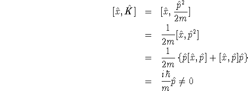
   2. To decide this, we need to work out the commutator of with :

      

      Since the commutator is not zero, the position and kinetic energy are not compatible.

4. 1. Using first-order perturbation theory, we have where is the particle-in-a-box energy and . In our case, . Thus, for the ground state,

      

      I called this quantity deltaE1 in my Maple session:
      

      > deltaE1:=2*V/L*int(sin(Pi*x/L)^2
      > *(x/L-1/2)^2,x=0..L);

      

      
      

      Thus

      

      Similarly, for the first excited state:

      

      
      

      > deltaE2:=2*V/L*int(sin(2*Pi*x/L)^2
      > *(x/L-1/2)^2,x=0..L);

      

      
      

      

   2. 

   3. To decide this, I first evaluated the numeric constant accompanying in deltaE1 and deltaE2:
      > evalf(deltaE1);

      

      > evalf(deltaE2);

      

      
      

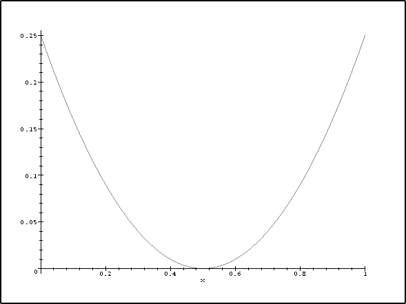
      deltaE2 ( ) is bigger. To decide why that is, I sketched the potential:
      > plot((x-1/2)^2,x=0..1);
      
      The energy of the n=2 level is most affected because the perturbation is greatest at the ends of the box and the electron density is greater at the ends for the n=2 state than for n=1 (which has its maximum density in the centre).
5. The probability is found by the integral

   

   where is whatever region of space we are interested in. For the 1s state,

   

   (I find it a little easier to keep track of all the brackets if I break it up into a product of three integrals than if I try to embed the integrals one into the other.)
   

   > 1/(Pi*a0^3)*int(exp(-r/a0)^2*r^2,r=0..2*a0)
   > *int(sin(theta),theta=0..Pi)
   > *int(1,phi=0..2*Pi);

   

   > simplify(");

   

   > evalf(");

   

   
   

   For the 2s state:

   

   
   

   > 1/(32*Pi*a0^3)
   > *int((2-r/a0)^2*exp(-r/(2*a0))^2*r^2,r=0..2*a0)
   > *int(sin(theta),theta=0..Pi)
   > *int(1,phi=0..2*Pi);

   

   > simplify(");

   

   > evalf(");

   

   
   

   Finally, to the probabilities of finding the electron between and in the two states, we just need to change the limits of integration:

   

   
   

   > 1/(Pi*a0^3)*int(exp(-r/a0)^2*r^2,r=2*a0..10*a0)
   > *int(sin(theta),theta=0..Pi)
   > *int(1,phi=0..2*Pi);

   

   > simplify(");

   

   > evalf(");

   

   
   

   

   
   

   > 1/(32*Pi*a0^3)
   > *int((2-r/a0)^2*exp(-r/(2*a0))^2*r^2,r=2*a0..10*a0)
   > *int(sin(theta),theta=0..Pi)
   > *int(1,phi=0..2*Pi);

   

   > simplify(");

   

   > evalf(");