Assignment 1 solutions

1. > int((x-2)*exp(-x^3),x=0..5);

   

   > evalf(%);

   

2. Note that both this and the following question involve the same function, so we might as well define it as a function:

   > ts := x -> tan(sin(x));

   

   > plot(ts,0..2*Pi);

   

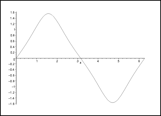
3. > solve(ts(x)=1,x);

   

Bonus:

There are some really easy solutions to this problem: The trigonometric functions are all -periodic, so is a solution for any integer n. For instance, is a solution. Surprisingly, this didn't occur to anyone. There's another class of ``easy'' solutions, and these are the ones which some of you found: when for integer n. We therefore want , with obvious solution . There's a problem with these solutions however: For any , |y|>1. The arcsine function is not defined over the real numbers for arguments of magnitude greater than unity. However, it is defined over the complex numbers and since I didn't specifically exclude complex solutions, these answers were technically correct and received credit.

I expected you to try to find the second solution which you can see on the graph of your function. Let's think about this for a second. The sine function looks like:

> plot(sin(x),x=0..2*Pi);

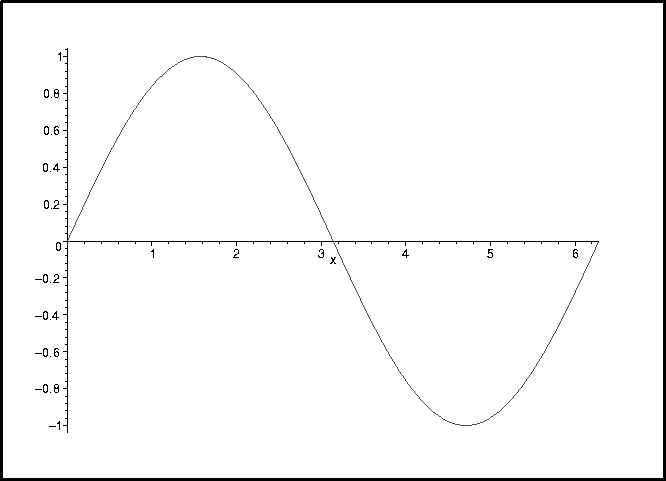
The reason why there are two solutions should now be clear: Between 0 and , passes through every value between 0 and 1 twice. We just have to find a solution to the equation with :

> u:=arcsin(Pi/4);

> solve(sin(u)=sin(u+a),a);

Maple finds two solutions, one of which is obvious and unhelpful (0). The other one is the one we want. Let's call the second solution of the equation w:

w:=arctan(Pi*sqrt(16-Pi^2)/(-8+Pi^2))+u;

Let's verify this result. First of all, we'll look at the floating-point value of w and make sure that it makes sense:

> evalf(w);

Comparing this value to the approximate solution found by examining the graph of , this looks right. Of course, that's not a very reliable way to go about verifying the answer. The right thing to do is to substitute w into the function ts and see what we get. It's possible to get Maple to show that this is an exact solution but it takes several steps and, after all, we're just verifying the result. It should be enough just to get the floating-point value of the function at w:

> evalf(ts(w));

For all intents and purposes, this is 1. The small difference is due to round-off error and is to be expected when doing finite-precision floating-point calculations.