Chemistry 3730 assignment 4 solutions

1. Define the wavefunctions and perturbing potential:
   

   > psi := (n,L,x) -> sqrt(2/L)*sin(n*Pi*x/L);

   

   > V := (L,x) -> Pi*h^2/(30*m*L^2)*sin(3*Pi*x/L);

   

   
   

   For n=1,
   

   > deltaE1 := int(psi(1,L,x)*V(L,x)*psi(1,L,x),x=0..L);

   

   
   

   For n=2,
   

   > deltaE2 := int(psi(2,L,x)*V(L,x)*psi(2,L,x),x=0..L);

   

   
   

   For n=3,
   

   > deltaE3 := int(psi(3,L,x)*V(L,x)*psi(3,L,x),x=0..L);

   

   
   

2. To answer this question, I'll use evalf() to convert the fractions to floating-point form:
   

   > evalf(deltaE1);

   

   > evalf(deltaE2);

   

   > evalf(deltaE3);

   

   
   

   The energy correction is greatest for n=2. Let's look at the probability densities and perturbing potential. To plot the densities, we'll pick a box of length 1. The density for n=1 looks like
   

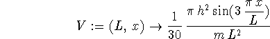
   > plot(psi(1,1,x)^2,x=0..1);

   

   
   

   For n=2, we have
   

   > plot(psi(2,1,x)^2,x=0..1);

   

   
   

   And, of course, for n=3,
   

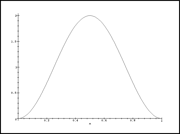
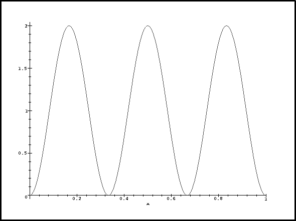
   > plot(psi(3,1,x)^2,x=0..1);

   

   
   

   The perturbing potential involves h and m, neither of which we really want to deal with directly, so let's plot :
   

   > plot(V(1,x)*m/h^2,x=0..1);

   

   
   

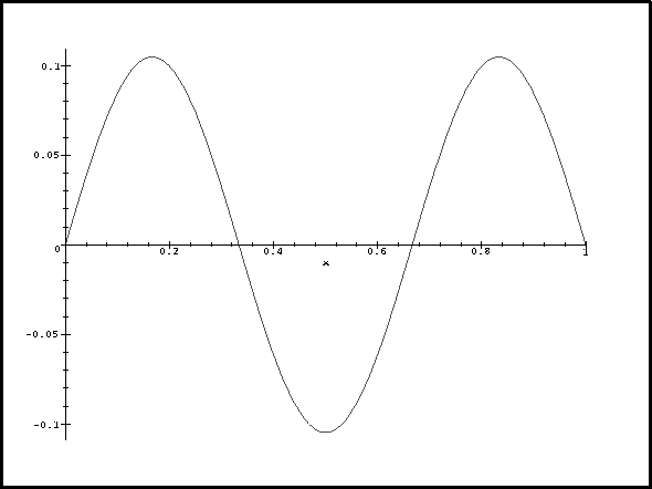
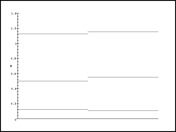
   Now let's think about this. For n=1, the probability density reaches a maximum in the middle where the perturbation is negative and large. This contributes a large negative term to the energy correction so deltaE1 is negative. For n=3, the probability density and perturbation have exactly the same periodicity. The contribution from the middle lobe exactly cancels that of one of the other two so we get a positive correction. We get the greatest correction for n=2 because the probability density has a node where the perturbation is most negative and is large where the perturbation reaches a maximum.

3. The energy levels of the particle in a box are given by
   

   > En := n -> n^2*h^2/(8*m*L^2);

   

   
   

   We want the energies of the unperturbed and perturbed system. For n=1,
   

   > evalf(En(1)); evalf(En(1)+deltaE1);

   

   

   
   

   For n=2,
   

   > evalf(En(2)); evalf(En(2)+deltaE2);

   

   

   
   

   For n=3,
   

   > evalf(En(3)); evalf(En(3)+deltaE3);

   

   

   
   

   I'm going to make my plot with Maple because I want an electronic document I can post on the web. It's far easier to do this by hand.
   

   > with(plots):
   > pa := plot([t,En(1)*m*L^2/h^2,t=0..1],0..2,0..1.2,
       labels=[``,`E `],xtickmarks=0):
   > pb := plot([t,En(2)*m*L^2/h^2,t=0..1],0..2,0..1.2,
       xtickmarks=0):
   > pc := plot([t,En(3)*m*L^2/h^2,t=0..1],0..2,0..1.2,
       xtickmarks=0):
   > pd := plot([t,(En(1)+deltaE1)*m*L^2/h^2,t=1..2],
       0..2,0..1.2,xtickmarks=0):
   > pe := plot([t,(En(2)+deltaE2)*m*L^2/h^2,t=1..2],
       0..2,0..1.2,xtickmarks=0):
   > pf := plot([t,(En(3)+deltaE3)*m*L^2/h^2,t=1..2],
       0..2,0..1.2,xtickmarks=0):
   > display(pa,pb,pc,pd,pe,pf);

   

   
   

   The unperturbed energy levels are on the left, the perturbed on the right.
4. The energy spacing between the ground state and first excited state increases so the wavelength of the corresponding photon decreases.