A brief example of neural data analysis using MATLAB

Edgar Bermudez, PhD

edgar.bermudez@uleth.ca

March 2013

Neural data analysis gives a better idea about the response or information processing/computation in a group of neurons.

Contents

Electrophysiology experiments

The recording system keeps track of

Silicon probes have recording sites (called tetrodes) with different configurations. Each probe has an array of shanks with recording sites. For the recordings in this experiment, one probe was inserted in S1 and another in mPFC.

Experiment description

The experiment consisted in recording neuronal data in anesthetized rats receving tactile stimulation under two conditions:

Neural data was recorded during periods of spontaneous (no stimulation) and evoked activity (where tactile stimulation was given) for both conditions.

Example of neuronal activity

There are different ways to represent neuronal activity, for this example, we choose to store spike information in a matrix with zeros and ones.

Important data structures in a electrophysiology recording

For this simple example we are going to analyze only a reduced sample of spike data (due to memory restrictions in the lab), however in a normal analysis we can combine LFP and spike data in recordings which can be very lengthy.

Plot experiment setup

1: SP ure, 2: stim ure, 3: SP ure, 5:SP Amph, 6:stim Amph, 7:SP Amph

If you are interested in looking at the same analysis for the whole recordings, check http://people.uleth.ca/~edgar.bermudez/matlab_class/html/matlabclass_analysis.html

Stimulus triggered activity

In order to have an idea about how neurons in the different areas respond to stimulation, we can display the stimulus triggered response (PSTH).

Load the data

datadir = 'C:\Users\edgar.bermudez\Documents\';
load([datadir 'LK10_sm' ]);

Neurons for S1 and PFC

pfc_nns = find( SpkEle<=8); % pfc neurons
s1_nns = find( SpkEle > 8); % s1 neurons
nr_pfc_nns = length( pfc_nns ); % number of pfc neurons

Extracting useful information In order to target our analysis, we divide and label the data to have a better control. For example, we need to know:

Some useful info

% Firing rate for S1 neurons during each stage
fr1 = mean(SpkCnt1(:,s1_nns));
fr2 = mean(SpkCnt2(:,s1_nns));
fr3 = mean(SpkCnt3(:,s1_nns));
% Firing rate for PFC neurons during each stage
fr4 = mean(SpkCnt1(:,pfc_nns));
fr5 = mean(SpkCnt2(:,pfc_nns));
fr6 = mean(SpkCnt3(:,pfc_nns));

Selection of active S1 neurons

select neurons with FR above threshold s1 and PFC

fr_th = 0.002;
act_s1nns = find( fr1 > fr_th & fr2 > fr_th & fr3 > fr_th);
act_pfcnns = find( fr4 > fr_th & fr5 > fr_th & fr6 > fr_th);

Slicing activity into trial locked time windows

% tactile stim trig activity before drug
f_tac1 = find(stim_sm==3);
f_tac1( find(diff( f_tac1 ) < 10 | diff( f_tac1 ) > 700)+1) = [];
w1=100; w2=750;
spk1=zeros(length(f_tac1),w1+w2+1,length(act_s1nns));
spk2=zeros(length(f_tac1),w1+w2+1,length(act_pfcnns));


for tr=2:length(f_tac1)-1
	spk1(tr,:,:)=SpkCnt2(f_tac1(tr)-w1:f_tac1(tr)+w2,s1_nns(act_s1nns));
    spk2(tr,:,:)=SpkCnt2(f_tac1(tr)-w1:f_tac1(tr)+w2,s1_nns(act_pfcnns));
end

% range of the reponse plots in ms
range = (-100:750)*3.2;

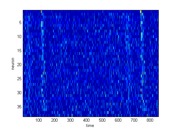
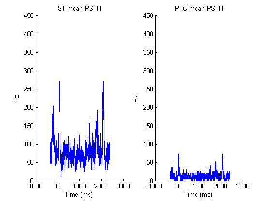
Plotting the response

figure();
title(['Neural response in urethane condition']);
imagesc(zscore(squeeze(mean(spk1)))');
xlabel('time');
ylabel('neuron');

figure();
subplot(1,2,1); hold on; title(['S1 mean PSTH']);
plot(range, 312.5*squeeze(mean(sum(spk1(:,:,:),3))));
ylim([0 450]);
xlabel('Time (ms)'); ylabel(' Hz ');
subplot(1,2,2); hold on; title(['PFC mean PSTH']);
plot(range, 312.5*squeeze(mean(sum(spk2(:,:,:),3))));
ylim([0 450]);
xlabel('Time (ms)'); ylabel(' Hz ');

Template matching

Template matching quantifies replay of temporal sequences of neuronal activity.

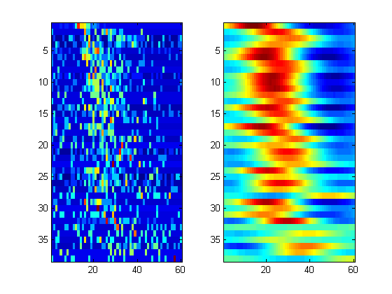
Template construction

Template is defined as the (summed evoked act - mean) / std average stim triggered activity of the S1 neurons

t_len = 60;
t_window = 101:100+t_len;
X = squeeze(sum(spk1(:,t_window,:),1))';

zs = zscore(X')';

figure('name','Template');
subplot(1,2,1); imagesc(zs);
% In order to have a less specific template, we smooth the activity pattern
% for every neuron
g_sigma = 20;
gs = normpdf(-g_sigma*2:g_sigma*2,0, g_sigma/2 )';

for n=1:size(zs,1)
	temp = zs( n, :);
	tmplt(n ,:) = conv2(  temp', gs, 'same');
end
template = tmplt(:,:);
subplot(1,2,2);
imagesc(template);

Matching

shift = 1;
num_windows = 37000;
norm_bef = zeros(1,num_windows); norm_aft = zeros(1,num_windows);

% take windows of activity to compare against our template
for j=1:num_windows
	winanalysis = 1+((j-1)*shift) : 1+((j-1)*shift)+t_len-1;
	% activity before stimulation
	tgt = SpkCnt1(winanalysis, s1_nns(act_s1nns))';
	% we normalize in the same way such windows
	tgt_z = zscore(tgt')';
	norm_aft(j) = dot(template(:), tgt_z(:)); % similarity comparison
	% activity after stimulation
	tgt = SpkCnt3(winanalysis, s1_nns(act_s1nns))';
	tgt_z = zscore(tgt')';
	norm_bef(j) = dot(template(:), tgt_z(:)); % similarity comparison
end

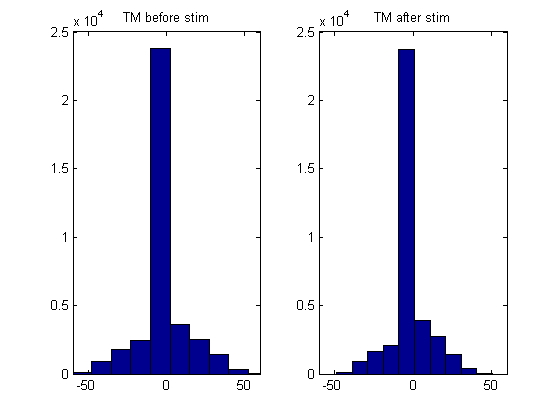
Results

We show the distribution of the TM signal before and after stimulation

figure();
subplot(1,2,1); hist(norm_bef);
title('TM before stim');
xlim([-60 60]);
subplot(1,2,2); hist(norm_aft);
title('TM after stim');
xlim([-60 60]);

References for further reading

Published with MATLAB® 7.14